Quickstart#

Note

This page presents the full workflow of tilepy, from the localization map to the observation schedule: display the sky map, extract the 90% credible region and its pixels, then run the scheduling. The companion notebook (button above) follows exactly these steps and can be run directly.

What you will see

What a HEALPix sky map looks like and how to display it.
How to extract the 90% probability and which pixels make it up.
How tilepy turns this region into a schedule of pointings.

The sky map#

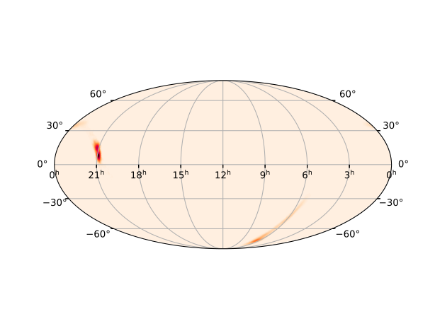
A localization map is a HEALPix map: the sky is tiled into pixels of equal area and each pixel i carries the probability that the source lies inside it. tilepy reads these maps internally (module tilepy.include.MapManagement), but to clearly visualize the starting point one can display it with ligo.skymap.

(Source code)

Tip

The figure above is produced by this snippet when the docs are built (it downloads only the small GW190728 skymap, a few MB). read_sky_map returns a flattened map (a single NSIDE); recent IGWN alerts are often multi-resolution (MOC): in that case use read_sky_map(url, moc=True). tilepy handles both formats automatically.

HEALPix resolution and order#

HEALPix is hierarchical: the sphere starts as 12 base pixels (order \(\ell = 0\)) and each pixel is recursively split into 4. The order (or level) \(\ell\) therefore sets the resolution:

\[\mathrm{NSIDE} = 2^{\ell}, \qquad N_\mathrm{pix} = 12\ \times \mathrm{NSIDE}^2 = 12 \cdot 4^{\ell}.\]

Every pixel covers the same solid angle:

\[\Omega_\mathrm{pix} = \frac{4\pi}{N_\mathrm{pix}} = \frac{41253\ \mathrm{deg}^2}{N_\mathrm{pix}}, \qquad \theta_\mathrm{pix} \approx \sqrt{\Omega_\mathrm{pix}} \approx \frac{58.6°}{\mathrm{NSIDE}}.\]

Worked example (\(\ell = 6\)): \(\mathrm{NSIDE} = 2^6 = 64\), \(N_\mathrm{pix} = 12\cdot64^2 = 49152\), \(\Omega_\mathrm{pix} = 41253/49152 \approx 0.84\ \mathrm{deg}^2\), \(\theta_\mathrm{pix} \approx 58.6/64 \approx 0.92°\).

Resolution as a function of the order#
\(\ell\)	NSIDE	\(N_\mathrm{pix}\)	Pixel area	Pixel size
6	64	49,152	\(\approx 0.84\ \mathrm{deg}^2\)	\(\approx 0.92°\)
8	256	786,432	\(\approx 0.052\ \mathrm{deg}^2\)	\(\approx 0.23°\)
9	512	3,145,728	\(\approx 0.013\ \mathrm{deg}^2\)	\(\approx 0.11°\)

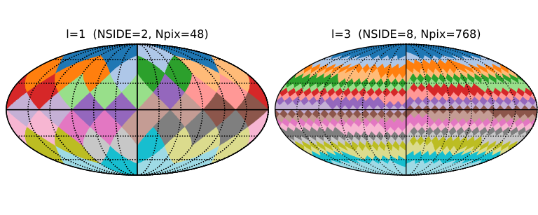
Going from \(\ell\) to \(\ell+1\) multiplies the number of pixels by 4 and halves the pixel size. This is the multi-resolution “tree” used by IGWN MOC maps: well-localized regions are stored at high \(\ell\), empty regions at low \(\ell\). The figure below (rendered at build time) shows the same sphere pixelized at two orders:

import numpy as np, healpy as hp
import matplotlib.pyplot as plt

fig = plt.figure(figsize=(8, 3.2))
for i, ns in enumerate([2, 8]):
    hp.mollview(np.arange(hp.nside2npix(ns)), sub=(1, 2, i + 1), cbar=False,
                cmap="tab20",
                title=f"l={int(np.log2(ns))}  (NSIDE={ns}, Npix={hp.nside2npix(ns)})")
    hp.graticule()

(Source code)

Important

tilepy works with two orders, configurable in the .ini file:

HRnside (high \(\ell\)) to integrate the probability inside a field of view precisely;
reducedNside (low \(\ell\)) to scan the sky quickly.

Extracting the 90% region#

Principle (greedy algorithm). Sort the pixels from most to least probable, accumulate their probability, and keep the first ones until the desired fraction is reached (here 0.9). The area is simply the number of retained pixels times the area of one pixel.

With healpy (pedagogical)

import numpy as np

order = np.argsort(prob)[::-1]      # decreasing sort
cumul = np.cumsum(prob[order])      # cumulative sum
pix_90 = order[cumul <= 0.90]       # pixels of the 90%

pix_area = hp.nside2pixarea(nside, degrees=True)
area_90 = len(pix_90) * pix_area
print(f"{len(pix_90)} pixels  ->  {area_90:.1f} deg²")

With tilepy

Once the map is loaded into a SkyMap object, the same computation is directly available:

skymap.getArea(0.9)          # area of the 90% region (deg²)
skymap.getPixIdArea(0.9)     # indices of the pixels in the region

And to retrieve the (RA, Dec) coordinates on a reduced grid — this is the list of positions the algorithm then scans:

from tilepy.include.PointingTools import GetRegionPixReduced
ra, dec, area = GetRegionPixReduced(prob, 0.9, reducedNside)

The scheduling process#

tilepy is driven by a .ini configuration file (telescope, visibility constraints, strategy) and an ObservationParameters object. We stay here on the simplest case: algorithm = 2D (probability integration) for a ground-based telescope.

Important

In 2D mode tilepy does not read any galaxy catalog, so there is nothing heavy to download (the GLADE+ catalog Gladeplus.h5 is only needed in 3D mode). Pass None for both the dataset directory and the catalog name.

What does GetSchedule do in 2D mode?

reads the map and computes the 90% region (previous section);
splits the night into observable dark-time windows at the site;
at each window, centers the field of view on the pixel with the highest probability still visible, adds up the probability contained in the FoV, then masks those pixels so they are not counted again;
repeats until maxRuns pointings (or until the probability above minProbcut is exhausted).

The result is a table of pointings SuggestedPointings_2DProbOptimisation.txt (columns Time[UTC], RA[deg], DEC[deg], PGW, …), together with the figures if doPlot = True.

Reading the produced schedule#

from astropy.table import Table
res = Table.read(
    "output/GW190728/PGinFoV/SuggestedPointings_2DProbOptimisation.txt",
    format="ascii")
print(res)
print("Total covered probability:", res["PGW"].sum())